Posts for Tag: interactive
Scaling the physical size of States in the US to reflect population size (animation)
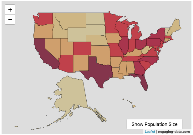
States sized to New Jersey’s population density
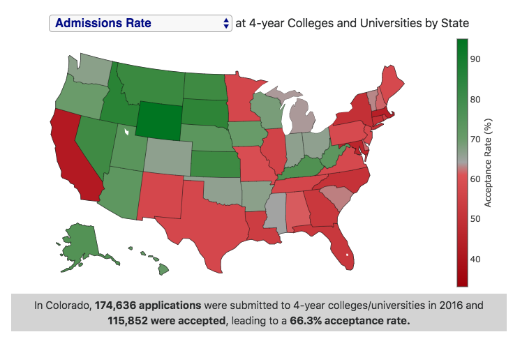
Choropleth maps are a pretty useful kind of map that colors distinct areas of the map (e.g. states, counties or countries) to reflect different numerical or categorical values. It is useful to show differences across geographic regions. I’ve been making a bunch of these recently (stressed states, bitcoin electricity consumption, college admissions). One of the issues that can be problematic with these maps is that some regions can be very large but only have very few people. If the choropleth map is tracking a intensity value (like CO2 emissions per capita), a large area with a high color value might visually indicate that total emissions (emissions per capita x # of people) is also high. In the US this is reflected in states like Alaska, Montana and Wyoming, which are large but have very few people.
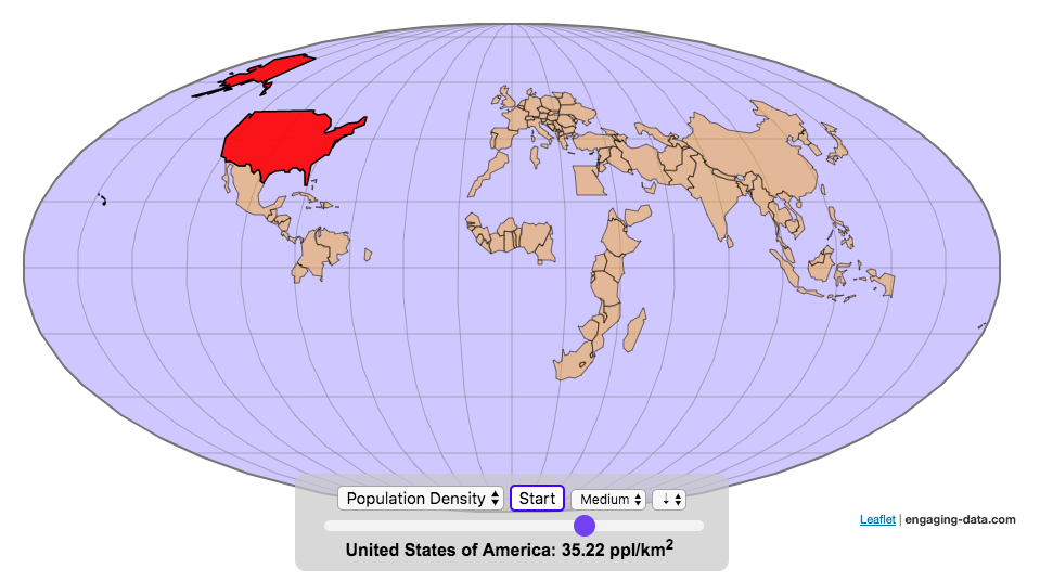
I decided to make a modified choropleth map (updated after learning that it’s called a cartogram) that scales the size of the states to be the proportional to the state’s population. States with larger populations show up as larger. This is equivalent to making each state have the same population density. Since New Jersey has the highest population density of any state in the US (1200 people/square mile), it stays the same size in this map and all the other states shrink, to reflect their lower population density. For example, California has a larger population than NJ (4.4x), but its physical size is about 20x larger. So California is shrunk to about 20% its original size to make its physical size 4.4x the size of NJ.
The states are also colored to show population as well (darker redder colors reflect larger population while yellow/beige reflects small populations).
States sized to California’s population density
Living in California, I decided to make another animation, this time with scaled to the density of California, so some states that are less dense will shrink, while others that are denser will grow. New Jersey grows quite a bit. Because many of the dense Northeast states grow a bit, I had to space them out (manually) so you could still see them otherwise they’d overlap too much.
Data Sources and Tools:
2015 population and population density data comes from Wikipedia and leaflet.js open source mapping library was used to create the maps. State outlines in geoJSON format come from leaflet. Javascript code was used to scale the coordinates of the geoJSON polygons to the appropriate size and animate the map.
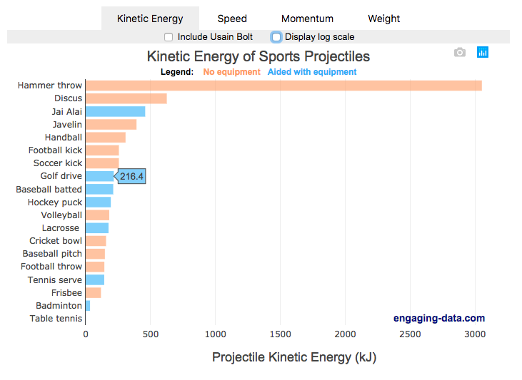
Speed and Kinetic Energy of Sports Pitches, Shots and Kicks
I’ve been playing (and watching) alot of soccer recently with the kids and it got me thinking about how hard the pros can kick the ball compared to us. This got me thinking about how much energy athletes can impart to a soccer ball and how that compares to balls and projectiles in other sports. This is not a scientific study, as I just googled the fastest pitch, shot, serve, kick, throw etc. from a variety of sports and the weight of the respective balls/projectiles to calculate their kinetic energy and momentum. I added in the stats for a (sort of) human projectile for comparison as well (Usain Bolt).
The graph is color coded so orange refers to projectiles that require no additional equipment, while the blue requires a bat or racket or club to aid in hitting the ball. You can toggle between log and linear scale on the x-axis to better see the differences between different projectiles.
The hammer throw is interesting because it far exceeds the kinetic energy and momentum of the other balls. If you watch a video of olympic hammer throws, you’ll see how much energy these very large, strong athletes are able to put into the throw. I think another aspect is that the top kinetic energy projectiles are all throws where there is significant acceleration of the projectile over a longer period of time rather than an instantaneous kick or hit.
Switching to the speed tab, all of the fastest projectiles are aided by equipment to achieve their very high speeds, but generally these projectiles have lower weights. This is also seen in the momentum tab, where the heavier projectiles are mostly unaided by equipment, probably because of the challenge of imparting enough momentum onto a heavy ball/projectile would require accelerating an even heavier racket/bat.
Equations and stuff
The equation for kinetic energy is \(E = {1\over2} mv^2\),
where E is kinetic energy (expressed in joules or kilojoules), m is mass and v is velocity (or speed).
The equation for momentum is \(P = mv\), where P is momentum.
The difference between momentum and kinetic energy is slightly tricky. The momentum rankings seem to prioritize the mass of the projectile while kinetic energy is a balance between speed (velocity) and mass. In kicking, throwing or hitting a ball/projectile, the player needs to put impart the energy into the ball. In a collision, total momentum of the system (player and ball) is conserved but kinetic energy is not, although total energy is (some energy may be “lost” as heat, sound, etc). In terms of being “hit” by the projectile, I believe that kinetic energy is probably more important than momentum for gauging the overall effect of the impact, but the total energy is not the only concern.The area over which the impact would occur is also important. Honestly, the table tennis (ping-pong) ball is the only one I think I’d be okay getting hit by (at least at these world record speeds).
Data sources and tools:
Mostly google for ball weights and trying to find some mention of the “fastest” throw or kick or whatever. Calculations are made using the equations above and plotted using Plot.ly javascript library.

Real Country Sizes Shown on Mercator Projection (Updated)
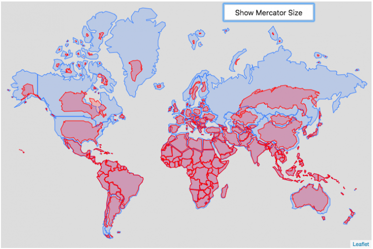
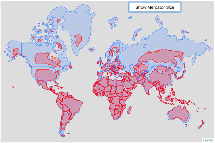
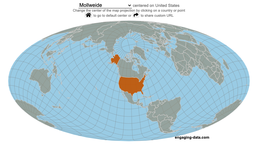
Hover or click on a country to see how much it shrinks from the Mercator projection size.
Check out some other engaging and interactive map dataviz:
I remember as a child thinking that Alaska was as large as 1/2 of the continental US. Later, however, I learned that while it is the largest state, it is actually only about 1/5 the size of the lower 48 states. My son has also remarked that Greenland is very big. And while it is very big, it’s nowhere near the size of the continent of Africa.
The map above shows the distortion in sizes of countries due to the mercator projection. Pressing on the button animates the country ‘shrinking’ to its actual size or ‘growing’ to the size shown on the mercator projection. It was inspired by a similar animation that I saw on reddit and decided I wanted to try to build the same thing.
The mercator projection is a commonly used projection on computer maps because it has perpendicular latitude and longitude lines (forming rectangles). It is formed by projecting the globe onto a cylinder A variant of the was adopted by Google maps, which helped establish it as the informal standard for web-based maps (although Google maps now also uses a globe view, instead of a map projection when zooming out to a very wide view).
Areas far from the equator are distorted in terms of their distances and are shown much larger than they actually are. This is one of the major issues with a projection of a globe onto a cylinder area. This is why Greenland, Russia and Canada shrink so much in height and width in the animation, they are fairly high in latitude in the Northern Hemisphere. Also important is that the closer you are to the poles, the more the distortion when a country is shown on the Mercator projection. Since longitude lines converge at the poles, but are parallel on a Mercator, the closer a part of a country is to the poles, the more that part will get stretched wider relative to a part of a country that is not as close to the poles. As a clear example, see what happens to the southern part of Australia, relative to the northern end. Similarly, the latitude lines also get further apart on a Mercator projection, while on a globe they stay equidistant. This means that the parts of countries that are nearer the poles will get taller, i.e. stretched out from a north-south perspective relative to parts of countries that are further from the poles. You can see this clearly in the northern ends of Russsia and Greenland, where the tops get smushed down.
This next graph shows each country plotted with their actual land area and apparent land area as shown on a Mercator projection. The further the countries are from the 1:1 line the greater the overestimate of their size from the Mercator (also color coded to be red). It is a logarithmic plot showing many different orders of magnitude in country size. The table also shows the top 10 countries whose size is overestimated (and the difference in land area in square kilometers or as a percentage reduction from the size in the Mercator projection).
As it shows, Greenland is the country that has the largest percent difference between its apparent size in a Mercator projection and it’s real size (it’s only about 1/4 of the apparent size). And Russia is the country with the largest absolute difference between these two sizes.
This is the original graph that keeps the shape of the countries exactly the same and just scales the size. This is incorrect because as you move towards the poles the distances between longitude lines decreases. As a result the tops (northern ends) of countries will shrink more than the bottoms (southern ends) of countries in the Northern Hemisphere and vice versa in the Southern Hemisphere.
Old map that changes sizes but incorrectly preserves the Mercator shape
Calculations:
I calculated the area in two ways, one assuming latitude and longitude are rectangular coordinates (i.e. Mercator projection) and the other was the actual area.
The new coordinates needed to draw the “real size” of the countries are derived by calculating the distance between the center of the country and each of the coordinates in the country’s shapefile. As you move towards the poles on a globe, the distance between longitude lines decreases as a function (cosine) of latitude. In a mercator projection, the longitude lines are shown as equi-distant regardless of latitude. In this calculation, we create a new set of coordinates by calculating the distance between the center of the polygon and each set of coordinates and change the coordinates to reflect the shrinking of distance between longitude lines as you head towards the poles.
In the previous version of this animation, I calculated the latitude and longitude coordinates for the outline of the “real” size by modifying the original latitude and longitude by the ratio of these two areas to draw the new smaller, “real” country size.
Data and tools: This visualization was made using the Leafletjs javascript mapping library and country shapefiles (converted to geojson).
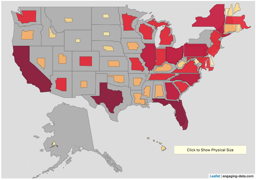
Bitcoin Energy Consumption – Does It Consume More Electricity Than Your State?

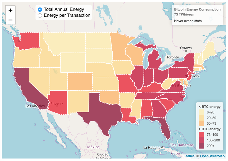
This visualization looks at the staggeringly high energy use of Bitcoin and puts it into context: comparing it to electricity usage of US states. Unfortunately for Bitcoin, high energy usage is an intended feature of the system, rather than an unintended consequence. This is because mining is an increasingly energy intensive process, based upon increasingly computationally intensive calculations that are performed on high powered computers and graphical processing units.
Currently, 28 out of 50 states plus the District of Columbia all have lower electricity consumption than estimated annual bitcoin electricity consumption (~73 TWh per year). These states are highlighted in variations of yellow. This is approximately equal to the average annual electricity usage across all US States. States with higher electricity consumption than bitcoin are highlighted in shades of red.
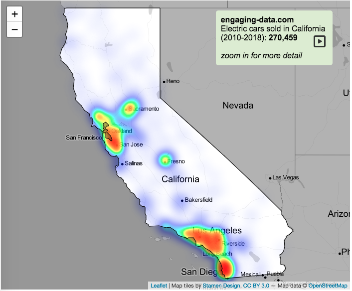
When dividing the total energy use (73 TWh) by the current number of transactions (93 million), we get an average energy consumption of 783 kWh per transaction. Click on the “Energy per Transaction” button to see this visualization. What’s crazy is that a transaction is simply a transfer of bitcoin between “wallets”, recording the transaction, and a validation of the process. There’s no good reason why verifying digital transactions should take this much energy, except that it was built into the fundamental process of validating and mining bitcoin. 783 kWh is larger than the monthly per capita electricity consumption in 10 US states. It could also drive you and your family over 2000 miles in an electric car (e.g. Tesla Model S).
I’m not expert enough in this area to know how much more energy consumption will rise into the future, but if crypto advocates’ predictions come true and bitcoin is used extensively, millions of transactions will occur per hour instead of per year and the price of bitcoin may rise much higher than it currently is. If the price rises, then miners will be willing to expend more energy to “mine” the more valuable bitcoin. Needless to say, this sounds like a very bad idea from an energy consumption and sustainability standpoint.
Data and Tools:
State energy data comes from the US Department of Energy. Estimates of Bitcoin energy use come from Digiconomist’s Bitcoin Energy Consumption Index. The choropleth map is visualized using javascript and the Leaflet.js library with Open Street Map tiles.
Scaling the physical size of States in the US to reflect population size (animation)
States sized to New Jersey’s population density
Choropleth maps are a pretty useful kind of map that colors distinct areas of the map (e.g. states, counties or countries) to reflect different numerical or categorical values. It is useful to show differences across geographic regions. I’ve been making a bunch of these recently (stressed states, bitcoin electricity consumption, college admissions). One of the issues that can be problematic with these maps is that some regions can be very large but only have very few people. If the choropleth map is tracking a intensity value (like CO2 emissions per capita), a large area with a high color value might visually indicate that total emissions (emissions per capita x # of people) is also high. In the US this is reflected in states like Alaska, Montana and Wyoming, which are large but have very few people.
I decided to make a modified choropleth map (updated after learning that it’s called a cartogram) that scales the size of the states to be the proportional to the state’s population. States with larger populations show up as larger. This is equivalent to making each state have the same population density. Since New Jersey has the highest population density of any state in the US (1200 people/square mile), it stays the same size in this map and all the other states shrink, to reflect their lower population density. For example, California has a larger population than NJ (4.4x), but its physical size is about 20x larger. So California is shrunk to about 20% its original size to make its physical size 4.4x the size of NJ.
The states are also colored to show population as well (darker redder colors reflect larger population while yellow/beige reflects small populations).
States sized to California’s population density
Living in California, I decided to make another animation, this time with scaled to the density of California, so some states that are less dense will shrink, while others that are denser will grow. New Jersey grows quite a bit. Because many of the dense Northeast states grow a bit, I had to space them out (manually) so you could still see them otherwise they’d overlap too much.
Data Sources and Tools:
2015 population and population density data comes from Wikipedia and leaflet.js open source mapping library was used to create the maps. State outlines in geoJSON format come from leaflet. Javascript code was used to scale the coordinates of the geoJSON polygons to the appropriate size and animate the map.
Speed and Kinetic Energy of Sports Pitches, Shots and Kicks
I’ve been playing (and watching) alot of soccer recently with the kids and it got me thinking about how hard the pros can kick the ball compared to us. This got me thinking about how much energy athletes can impart to a soccer ball and how that compares to balls and projectiles in other sports. This is not a scientific study, as I just googled the fastest pitch, shot, serve, kick, throw etc. from a variety of sports and the weight of the respective balls/projectiles to calculate their kinetic energy and momentum. I added in the stats for a (sort of) human projectile for comparison as well (Usain Bolt).
The graph is color coded so orange refers to projectiles that require no additional equipment, while the blue requires a bat or racket or club to aid in hitting the ball. You can toggle between log and linear scale on the x-axis to better see the differences between different projectiles.
The hammer throw is interesting because it far exceeds the kinetic energy and momentum of the other balls. If you watch a video of olympic hammer throws, you’ll see how much energy these very large, strong athletes are able to put into the throw. I think another aspect is that the top kinetic energy projectiles are all throws where there is significant acceleration of the projectile over a longer period of time rather than an instantaneous kick or hit.
Switching to the speed tab, all of the fastest projectiles are aided by equipment to achieve their very high speeds, but generally these projectiles have lower weights. This is also seen in the momentum tab, where the heavier projectiles are mostly unaided by equipment, probably because of the challenge of imparting enough momentum onto a heavy ball/projectile would require accelerating an even heavier racket/bat.
Equations and stuff
The equation for kinetic energy is \(E = {1\over2} mv^2\),
where E is kinetic energy (expressed in joules or kilojoules), m is mass and v is velocity (or speed).
The equation for momentum is \(P = mv\), where P is momentum.
The difference between momentum and kinetic energy is slightly tricky. The momentum rankings seem to prioritize the mass of the projectile while kinetic energy is a balance between speed (velocity) and mass. In kicking, throwing or hitting a ball/projectile, the player needs to put impart the energy into the ball. In a collision, total momentum of the system (player and ball) is conserved but kinetic energy is not, although total energy is (some energy may be “lost” as heat, sound, etc). In terms of being “hit” by the projectile, I believe that kinetic energy is probably more important than momentum for gauging the overall effect of the impact, but the total energy is not the only concern.The area over which the impact would occur is also important. Honestly, the table tennis (ping-pong) ball is the only one I think I’d be okay getting hit by (at least at these world record speeds).
Data sources and tools:
Mostly google for ball weights and trying to find some mention of the “fastest” throw or kick or whatever. Calculations are made using the equations above and plotted using Plot.ly javascript library.
Real Country Sizes Shown on Mercator Projection (Updated)
Hover or click on a country to see how much it shrinks from the Mercator projection size.
Check out some other engaging and interactive map dataviz:
I remember as a child thinking that Alaska was as large as 1/2 of the continental US. Later, however, I learned that while it is the largest state, it is actually only about 1/5 the size of the lower 48 states. My son has also remarked that Greenland is very big. And while it is very big, it’s nowhere near the size of the continent of Africa.
The map above shows the distortion in sizes of countries due to the mercator projection. Pressing on the button animates the country ‘shrinking’ to its actual size or ‘growing’ to the size shown on the mercator projection. It was inspired by a similar animation that I saw on reddit and decided I wanted to try to build the same thing.
The mercator projection is a commonly used projection on computer maps because it has perpendicular latitude and longitude lines (forming rectangles). It is formed by projecting the globe onto a cylinder A variant of the was adopted by Google maps, which helped establish it as the informal standard for web-based maps (although Google maps now also uses a globe view, instead of a map projection when zooming out to a very wide view).
Areas far from the equator are distorted in terms of their distances and are shown much larger than they actually are. This is one of the major issues with a projection of a globe onto a cylinder area. This is why Greenland, Russia and Canada shrink so much in height and width in the animation, they are fairly high in latitude in the Northern Hemisphere. Also important is that the closer you are to the poles, the more the distortion when a country is shown on the Mercator projection. Since longitude lines converge at the poles, but are parallel on a Mercator, the closer a part of a country is to the poles, the more that part will get stretched wider relative to a part of a country that is not as close to the poles. As a clear example, see what happens to the southern part of Australia, relative to the northern end. Similarly, the latitude lines also get further apart on a Mercator projection, while on a globe they stay equidistant. This means that the parts of countries that are nearer the poles will get taller, i.e. stretched out from a north-south perspective relative to parts of countries that are further from the poles. You can see this clearly in the northern ends of Russsia and Greenland, where the tops get smushed down.
This next graph shows each country plotted with their actual land area and apparent land area as shown on a Mercator projection. The further the countries are from the 1:1 line the greater the overestimate of their size from the Mercator (also color coded to be red). It is a logarithmic plot showing many different orders of magnitude in country size. The table also shows the top 10 countries whose size is overestimated (and the difference in land area in square kilometers or as a percentage reduction from the size in the Mercator projection).
As it shows, Greenland is the country that has the largest percent difference between its apparent size in a Mercator projection and it’s real size (it’s only about 1/4 of the apparent size). And Russia is the country with the largest absolute difference between these two sizes.
This is the original graph that keeps the shape of the countries exactly the same and just scales the size. This is incorrect because as you move towards the poles the distances between longitude lines decreases. As a result the tops (northern ends) of countries will shrink more than the bottoms (southern ends) of countries in the Northern Hemisphere and vice versa in the Southern Hemisphere.
Old map that changes sizes but incorrectly preserves the Mercator shape
Calculations:
I calculated the area in two ways, one assuming latitude and longitude are rectangular coordinates (i.e. Mercator projection) and the other was the actual area.
The new coordinates needed to draw the “real size” of the countries are derived by calculating the distance between the center of the country and each of the coordinates in the country’s shapefile. As you move towards the poles on a globe, the distance between longitude lines decreases as a function (cosine) of latitude. In a mercator projection, the longitude lines are shown as equi-distant regardless of latitude. In this calculation, we create a new set of coordinates by calculating the distance between the center of the polygon and each set of coordinates and change the coordinates to reflect the shrinking of distance between longitude lines as you head towards the poles.
In the previous version of this animation, I calculated the latitude and longitude coordinates for the outline of the “real” size by modifying the original latitude and longitude by the ratio of these two areas to draw the new smaller, “real” country size.
Data and tools: This visualization was made using the Leafletjs javascript mapping library and country shapefiles (converted to geojson).
Bitcoin Energy Consumption – Does It Consume More Electricity Than Your State?
This visualization looks at the staggeringly high energy use of Bitcoin and puts it into context: comparing it to electricity usage of US states. Unfortunately for Bitcoin, high energy usage is an intended feature of the system, rather than an unintended consequence. This is because mining is an increasingly energy intensive process, based upon increasingly computationally intensive calculations that are performed on high powered computers and graphical processing units.
Currently, 28 out of 50 states plus the District of Columbia all have lower electricity consumption than estimated annual bitcoin electricity consumption (~73 TWh per year). These states are highlighted in variations of yellow. This is approximately equal to the average annual electricity usage across all US States. States with higher electricity consumption than bitcoin are highlighted in shades of red.
When dividing the total energy use (73 TWh) by the current number of transactions (93 million), we get an average energy consumption of 783 kWh per transaction. Click on the “Energy per Transaction” button to see this visualization. What’s crazy is that a transaction is simply a transfer of bitcoin between “wallets”, recording the transaction, and a validation of the process. There’s no good reason why verifying digital transactions should take this much energy, except that it was built into the fundamental process of validating and mining bitcoin. 783 kWh is larger than the monthly per capita electricity consumption in 10 US states. It could also drive you and your family over 2000 miles in an electric car (e.g. Tesla Model S).
I’m not expert enough in this area to know how much more energy consumption will rise into the future, but if crypto advocates’ predictions come true and bitcoin is used extensively, millions of transactions will occur per hour instead of per year and the price of bitcoin may rise much higher than it currently is. If the price rises, then miners will be willing to expend more energy to “mine” the more valuable bitcoin. Needless to say, this sounds like a very bad idea from an energy consumption and sustainability standpoint.
Data and Tools:
State energy data comes from the US Department of Energy. Estimates of Bitcoin energy use come from Digiconomist’s Bitcoin Energy Consumption Index. The choropleth map is visualized using javascript and the Leaflet.js library with Open Street Map tiles.
Recent Comments