Posts for Tag: calculator
Compound Interest and Stock Returns Calculator
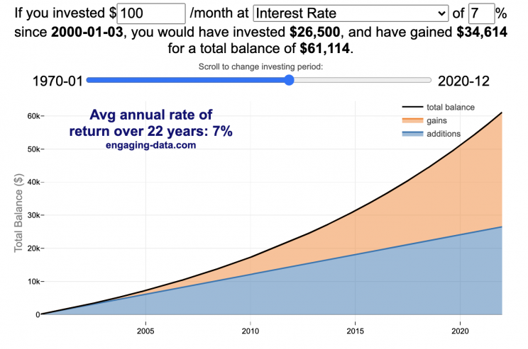
Calculate returns on regular, periodic investments
This calculator lets you visualize the value of investing regularly. It lets you calculate the compounding from a simple interest rate or looking at specific returns from the stock market indexes or a few different individual stocks.
Instructions
- Enter the amount of money to be invested monthly
- Choose to use an interest rate (and enter a specific rate) or
- Choose a stock market index or individual stock
- Use the slider to change the initial starting date of your periodic investments – You can go as far back as 1970 or the IPO date of the stock if it is later than that.
- Use the “Generate URL to Share” button to create a special URL with the specific parameters of your choice to share with others – the URL will appear in your browser’s address bar.
You can hover over the graph to see the split between the money you invested and the gains from the investment. In most cases (unless returns are very high), initially the investments are the large majority of the total balance, but over time the gains compound and eventually, it is those gains rather than the initial investments that become the majority of the total.
Some of the tech stocks included in the dropdown list have very high annualized returns and thus the gains quickly overtake the additions as the dominant component of the balance and you can make a great deal of money fairly quickly.
It becomes clearer as you move the slider around, that longer investing time periods are the key to increasing your balance, so building financial prosperity through investing is generally more of a marathon and not really a sprint. However, if you invest in individual stocks and pick a good one, you can speed up that process, though it’s not necessarily the most advisable way to proceed. Lots of people underperform the market (i.e. index funds) or even lose money by trying to pick big winners.
Understanding the Calculations
Calculating compound returns is relatively easy and is just a matter of consecutively multiplying the return. If the return is 7% for 5 years, that is equal to multiplying 1.07 five times, i.e. 1.075 = 1.402 (or a 40.2% gain).
In this case, we are adding additional investments each month but the idea is the same. Take the amount of money (or value of shares) and multiply by the return (>1 if positive or <1 for negative returns) after each period of the analysis.
Sources and Tools:
Stock and index monthly data is downloaded from Yahoo! finance is downloaded regularly using a python script.
The graph is created using the open-source Plotly javascript visualization library, as well as HTML, CSS and Javascript code to create interactivity and UI.

Early Retirement Calculators and Tools
Interested in Early Retirement or FIRE (Financial Independence to Retire Early)?
Here are some interactive and educational planning tools that I developed to help you understand the concepts of FIRE and calculate how long it will take to achieve retirement and how likely you are to survive retirement. Click on the tools below to try them out.
Financial Independence Calculators
Regardless of where you are on your path to FIRE, there are several types of tools that are useful:
Planning to get to retirement
How long and how safe will your retirement be?
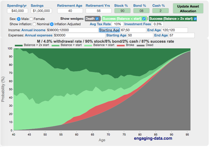
Rich, Broke or Dead? Will your Money Last Through Early Retirement?
Simulating retirement portfolio survival probability and human longevity
Determining the appropriate withdrawal rate (i.e. is 4% best?)
Understanding portfolio simulations and historical cycles
Interactive tool lets you explore the concept of historical simulations and understand how to determine a safe withdrawal rate
Tracking Progress to Retirement Target
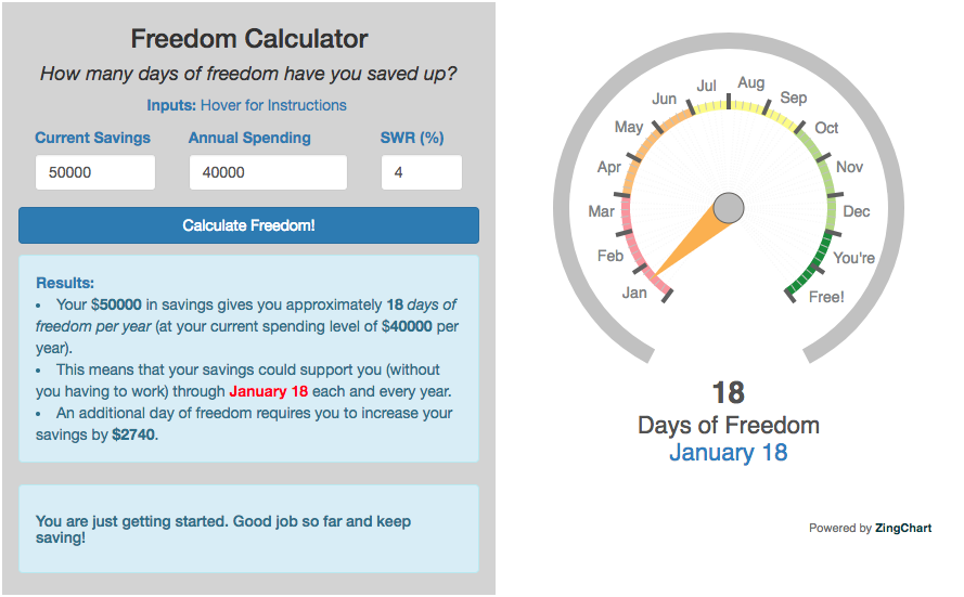
Financial freedom calculator / calendar
Track your progress to retirement by calculating days of “freedom”, the number of days your savings could support you per year
These tools all focus on the concept of FIRE. FIRE is the concept that revolves around saving and investing to achieve Financial Independence (FI) and to potentially Retire Early (RE). One of the core concepts is that once you can save up enough money, you can retire by withdrawing a fraction of this money annually to cover your living expenses. Other important topics related to this core concept have to do with reducing spending so you can save money and investing so your money can grow and sustain your retirement over many decades.
Other visualizations and tools related to Financial Independence
These tools relate to taxes and stock market returns.
Calculating Returns from Periodic Investments
Visualizing Market Returns
Understanding Market Timing
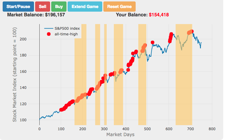
Market Timing Game
How difficult is it to time the stock market?
Income Taxes
Income Tax Bracket Calculator
Tax bracket calculator to visualize how income and capital gains taxed
Data Sources and Tools:
See the individual tool to learn more about how it was made.
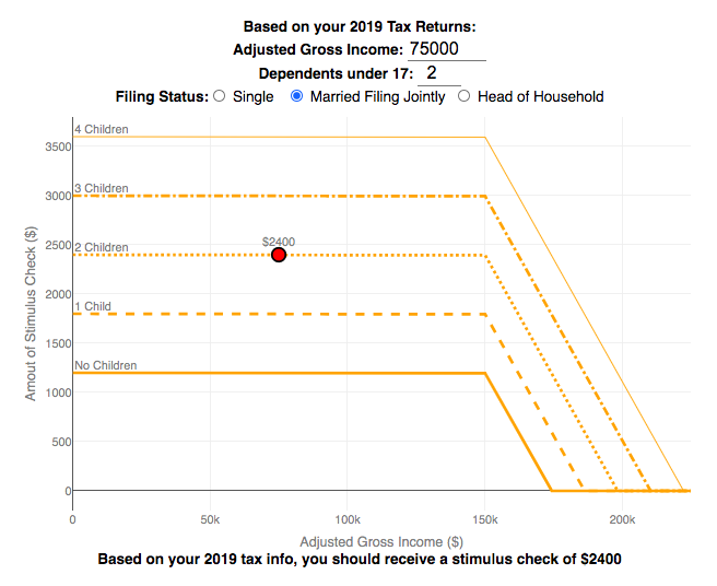
Stimulus Check Calculator (Late 2020 & Early 2021)

How much money can you expect in your stimulus check?
Updated to include the $1400 stimulus payment per adult and dependent in March 2021.
Use this stimulus check calculator to figure out how much you will receive in your thrid stimulus check.
On December 21, 2020, Congress passed a $900 billion dollar stimulus package in response to the COVID pandemic. The bill authorizes economic assistance to Americans in the amount of $600 per person subject to income limits. It also includes expanded unemployment benefits, rental assistance and an extension to the eviction ban. This calculator helps you calculate the amount of stimulus check that you can expect to receive based on your 2019 tax return filing status, adjusted gross income and number of dependents under 17.
Changing the inputs to the calculator, will show you how your expected stimulus check amount will change. The graph shows for a giving filing status (single, married filing jointly or head of household) how the stimulus check amount will change as a function of income and number of children. You can share a URL with specific parameters included
Sounds like some checks may even get to folks at the end of December and many more will get them in January 2021.
On March 5, congress passed the American Rescue Plan which includes $1400 payments for all Americans. The phase out of this stimulus check is different in that over a $10000 range the stimulus goes from 100% to 0% at the phase out threshold, no matter how many dependents you have. This changes things significantly as you’ll see in the calculator.
Sources and Tools:
The stimulus check calculator is made using javascript and the plotly open source graphing library. It is based on news reports of the expected stimulus amounts and income thresholds.
Greenhouse gas emissions from airplane flights

Traveling by airplane produces significant greenhouse gas emissions
Flying in an airplane is likely the most greenhouse gas intensive activity you can do. In a few short hours, you can can travel thousands of miles across the continent or ocean. It takes a large amount of fossil-fuel energy (oil) to lift an 80+ ton airplane off the ground and propel it at 600 miles per hour through the air. Every hour of travel (in a Boeing 737) consumes around 750 gallons of jet fuel.
Even when dividing the fuel usage across all of the passengers (and cargo) of an aircraft, airplane travel consumes a significant amount of fuel per passenger. The fuel economy is estimated to be about the same as a fairly efficient hybrid car driven by one person (60-70 passenger miles per gallon). However, because you can go 10 times faster and much further more easily than you would in a car, airline travel can, on an absolute basis, emit larger amounts of greenhouse gases. In fact, an individual passenger’s share of emissions from a single airplane flight can exceed the annual average greenhouse gas emissions per capita from a number of countries (and the global average).
The following flight calculator and data visualization shows the miles and emissions produced per passenger by a airplane trip that you can specify. Choose two airports that you are interested in and click the “Calculate Flight Emissions” button to see the emissions associated with a round-trip flight between these two cities. The map will show you the flight route and also shows you the countries in the world where this one single round-trip flight produces more emissions per passenger than the average resident does in one year from all sources (annual per capita emissions).
In addition to individual countries, the tool also compares the flight’s per passenger emissions to the global average emissions per capita in 2017 (4.91 tonnes) and the emissions required to achieve a 22℃ climate stabilization in 2030 (3.08 tonnes) and in 2050 (1.37 tonnes). These 2030 and 2050 numbers are based on an International Energy Agency scenario.
Calculations of Airplane Emissions
The emissions calculated by this calculator are based on calculations from myclimate.org, a non-profit environmental organization.
The fuel consumption of a jet depends on the size of the aircraft and distance traveled, but takeoff and climbing to cruising altitude are particularly fuel-intensive. On shorter flights, the takeoff and initial climb will constitute a greater proportion of the total flight time so fuel consumption per mile will be higher than on longer (e.g. international) flights.
The detailed methodology is described in more detail in this document.
In addition to emissions of CO2 from the burning of jet fuel, jets also emit other gases (including methane, NOx, and water vapor) which can also contribute to warming (also known as “radiative forcing”). Because the emissions are occurring at high altitude, these gases can have different impacts than those at lower altitude. A number of studies have estimated the impact of these other gases can significantly contribute to the overall radiative forcing and have somewhere between 1.5 and 3 times the impact that the CO2 alone would. A number of studies, including the myclimate calculator use a factor of 2 to account for these non-CO2 gases and their warming impact, and that is what is used in this calculator as well.
Unlike cars, trucks and trains, it is much harder to power airplanes with batteries and electricity and producing low-carbon jet fuels from biomass is proving very challenging.
In order to achieve climate stabilization at 2 degrees C, global emissions need to basically go to zero over the next 40 years. With a growing global population, this means that the allowable emissions per person will shrink rapidly over these coming decades.
Ultimately, while aviation is a small part of global greenhouse gas emissions, it is a larger part of emissions in richer countries (i.e. if you are reading/viewing this post). And there are many in these richer countries who fly a disproportionate amount and therefore contribute a disproportionate amount of emissions. Hopefully, putting airplane travel in this context can help us better understand the impact of our actions and choices and maybe even change behavior for some.
Tools and Data Sources
The calculator estimates flight emissions based on the myclimate carbon footprint calculator. Data for CO2 emissions by country was downloaded from the European Commissions’s Emissions Database for Global Atmospheric Research. The map was built using the leaflet open-source mapping library in javascript.

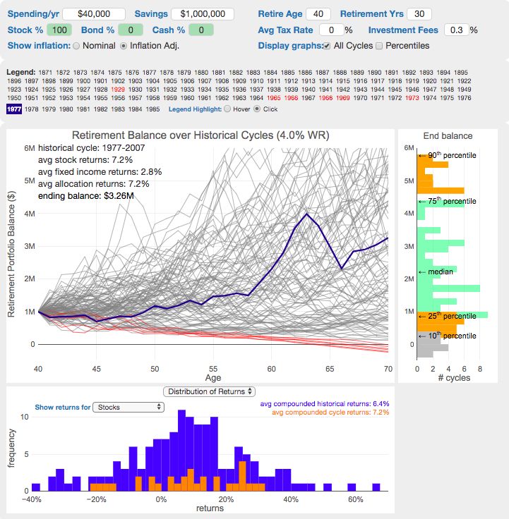
The 4% Rule, Trinity Study and Safe Withdrawal Rates Calculator

This 4% rule early retirement calculator is designed to help you learn about safe withdrawal rates for early retirement withdrawals and the 4% rule. Use it with your own numbers to determine how much money you can withdraw in retirement and how long your money will last.
UPDATE: I’ve updated the market data to include annual data up to and including 2023.
Instructions for using the calculator:
This calculator is designed to let you learn as you play with it. Tweaking inputs and assumptions and hovering and clicking on results will help you to really gain a feel for how withdrawal rates and market returns affect your chance of retirement success (i.e. making it through without running out of money).
Inputs You Can Adjust:
- Spending and initial balance – This will affect your withdrawal rate. The withdrawal rate is really the only thing that is important (doubling spending and retirement savings will still yield the same success rate).
- Asset allocation – Raise or lower your risk tolerance by holding more or less stock vs bonds
- Adjust retirement length – This affects the number of historical cycles that are used in the simulation, but also increases risk of failure.
- Add tax rates and investment fees – these will put a drag (i.e. lower) market returns and lower success rates
Options for Visualization:
- Display all cycles – this is the mess of spaghetti like curves that show all historical cycle simulations
- Display percentiles – this aggregates the simulations into percentiles to show most likely outcomes
- Hover/Click on legend years – this will allow you to highlight a single historical cycle (you can also use the arrow keys to step through historical cycles)
- Bottom graph can show either the sequence of returns (with average returns in 5 year periods) for a single historical cycle or distributions of returns in our historical data (1871 to 2016) and a single historical cycle. You can choose to look at returns for stocks, bonds or your specific asset allocation.
- The graph on the right shows a histogram of the ending balance of each historical cycle and color codes them to show percentiles.
What is the 4% Rule?
The 4% rule is a “rule of thumb” relating to safe retirement withdrawals. It states that if 4% of your retirement savings can cover one years worth of retirement spending (an alternative way to phrase it is if you have saved up 25 times your annual retirement spending), you have a high likelihood of having enough money to last a 30+ year retirement. A key point is that the probabilities shown here are just historical frequencies and not a guarantee of the future. However, if your plan has a high success rate (95+%) in these simulations, this implies that retirement plan should be okay unless future returns are on par with some of the worst in history.
The overall goal of this rule and analysis is identifying a “safe withdrawal rate” or SWR for retirement. A withdrawal rate is the percentage of your money that you withdraw from your retirement savings each year. If you’ve saved up $1 million and withdraw $100,000 each year, that is a 10% withdrawal rate.
The “safe” part of the withdrawal rate relates to the fact that if your investments generally grow by more than your annual spending, then your retirement savings should last over the length of your retirement. But average returns do not tell the whole story as the sequence of returns also plays a very important role, as will be discussed later.
One way to test this is through a backtesting simulation which forms the basis for the “Trinity Study”.
What is the Trinity Study?
The “Trinity Study” is a paper and analysis of this topic entitled “Retirement Spending: Choosing a Sustainable Withdrawal Rate,” by Philip L. Cooley, Carl M. Hubbard, and Daniel T. Walz, three professors at Trinity University. This study is a backtesting simulation that uses historical data to see if a retirement plan (i.e. a withdrawal rate) would have survived under past economic conditions. The approach is to take a “historical cycle”, i.e. a series of years from the past and test your retirement plan and see if it runs out of money (“fails”) or not (“survives”).
How do you test withdrawal rate?
Given modern equity and bond market data only stretches back about 150 years, there is some, but not a huge amount of data to use in this simulation. One example of a 30 year historical cycle would be 1900 to 1930, and another is 1970 to 2000. The Trinity study and this calculator tests withdrawal rates against all historical periods from 1871 until the present (e.g. 1871 to 1901, 1872 to 1902, 1873 to 1903, . . . . 1986 to 2016). Then across this 115 different historical cycles, it determines how many of these survived and how many failed.
The thinking is that if your retirement plan can survive periods that include recessions, depressions, world wars, and periods of high inflation, then perhaps it can survive the next 30-50 years.
The 4% rule that comes out of these studies basically states that a 4% withdrawal rate (e.g. $40,000 annual spending on a $1,000,000 retirement portfolio) will survive the vast majority of historical cycles (~96%). If you raise your withdrawal rate, the rate of failure increases, while if you lower your withdrawal rate, your rate of failure decreases.
The goal of this tool is to help you understand the mechanics of the a historical cycle simulation like was used in the Trinity Study and how the 4% rule came to be. This understanding can help you better plan for retirement with the uncertainty that goes along with planning 30+ years into the future. If you want to also see how longevity and life expectancy play a role in retirement planning, you can take a look at the Rich, Broke and Dead calculator.
This post and tool is a work in progress. I have a number of ideas that I will implement and add to it to help improve the visualization and clarity of these concepts.
If 4% is a conservative rate, what is the maximum withdrawal rate?
The future is unlikely to be identical to any of the set of historical cycles that are used in this simulation. And yet, there are enough years of data that there are a fairly large set of possible outcomes from running a simulation with this input data. One way to understand this variation is to see in the main graph above that the ending balance can potentially vary by more than $5 million dollars on an inflation adjusted basis on a starting balance of $1 million.
Another way to see this same variation in market returns is by looking at maximum withdrawal rate. This is the highest amount that you could withdraw annually over your retirement and (just barely) not run out of money by the end of your retirement.
This graph shows the maximum withdrawal rate for a given historical cycle (i.e. 1871 to 1901). For example, in the 1871 to 1901 30 year historical cycle, you could have used an 8.8% withdrawal rate (inflation adjusted $80,000 withdrawal annually on a $1 million initial investment balance) and not run out of money. This is because the sequence of market (stock and bond) returns in this historical cycle were able to (barely) outpace the rate of withdrawals at the end of the 30 year retirement period. Many other cycles show lower successful withdrawal rates, because those cycles had poorer sequences of returns, while some had higher maximum withdrawal rates.
The graph also highlights those cycles that show a maximum withdrawal rate below 4% in red, while all others are shown in green. Most of these withdrawal rates are well over 4%, with some quite a bit higher. This again shows that if the future is somewhat like one of these historical cycles, most likely a 4% withdrawal rate will be enough for you to retire without running out of money and that it is likely that you could end up with more money than you started.
Data source and Tools Historical Stock/Bond and Inflation data comes from Prof. Robert Shiller. Javascript is used to create the interactive calculator tool and the create the code in the simulations to test each historical cycle and aggregate the results, and graphed using Plot.ly open-source, javascript graphing library.
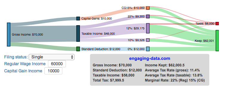
Visual Guide to Understanding Marginal Tax Rates
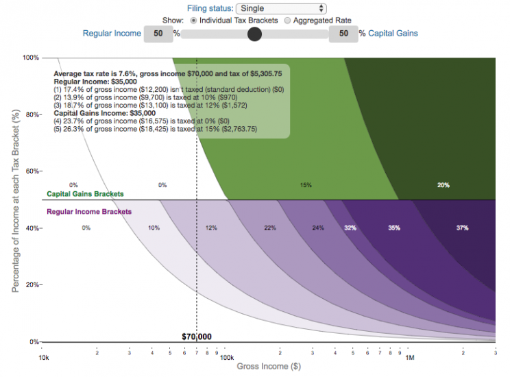
What is a marginal tax rate?
There is a fair amount of confusion about what a marginal tax rate is and how it affects how much tax you would owe the government on a certain amount of income. These graphs are here to help you better understand the difference between a marginal and average tax rate and to easily calculate these rates for specific examples in the US context. This tool only looks at US Federal Income taxes and ignores state, local and Social Security/Medicare taxes.
Marginal tax rates are the rate at which an additional dollar of income will be taxed at. There are different tax brackets (each with its own marginal rate) depending on which dollar of income you are looking at. This is very different from the Average (or effective) tax rate that is the result of applying these marginal tax rates across all of your income.
**Click Here to view other financial-related tools and data visualizations from engaging-data**
Instructions for using the visual tax calculator:
- Select filing status: Single, Married Filing Jointly or Head of Household. For more info on these filing categories see the IRS website
- Select percentage of regular income vs capital gains income. Regular income is wage or employment income and is taxed at a higher rate than capital gains income. Capital gains income is typically investment income from the sale of stocks or dividends and taxed at a lower rate than regular income.
- Move your cursor or click on the graph to select a specific income Make sure you note that the x-axis is a logarithmic-scale, meaning that income grows exponentially as you move to the right.
- Choose your graph preference One graph (Individual Tax Brackets) shows the individual tax brackets and how much of your income is taxed at the different marginal rates. The other graph (Aggregate Rates) shows the net result of applying the different rates to get your effective rate.
One of the most interesting things is to vary the proportion of regular income vs capital gains taxes. Generally, wealthier households earn a greater fraction of their income from capital gains and as a result of the lower tax rates on capital gains, these household pay a lower effective tax rate than those making an order of magnitude less in overall income.
Here are two tables that lists the marginal tax brackets in the United States in 2019 that form the basis of the calculations in the calculator. 2018’s numbers are pretty similar.
US Tax Brackets and Rates for 2019
Rate
Single
Taxable Income Over
Married Filing Joint
Taxable Income Over
Heads of Households
Taxable Income Over
10%
$0
$0
$0
12%
$9,700
$19,400
$13,850
22%
$39,475
$78,950
$52,850
24%
$84,200
$168,400
$84,200
32%
$160,725
$321,450
$160,700
35%
$204,100
$408,200
$204,100
37%
$510,300
$612,350
$510,300
You can see that tax rates are much lower for capital gains in the table below than for regular income (table above).
Capital Gains Brackets for 2019
Single
Capital Gains Over
Married Filing Jointly
Capital Gains Over
Heads of Households
Capital Gains Over
0%
$0
$0
$0
15%
$39,375
$78,750
$52,750
20%
$434,550
$488,850
$461,700
For those not visually inclined, here is a written description of how to apply marginal tax rates. The first thing to note is that the income shown here in the graphs is taxable income, which simply speaking is your gross income with deductions removed. The standard deduction for 2019 range from $12,200 for Single filers to $24,400 for Married filers.
- If you are single, all of your regular taxable income between 0 and $9,700 is taxed at a 10% rate. This means that your all of your gross income below $12,200 is not taxed and your gross income between $12,200 and $21,900 is taxed at 10%.
- If you have more income, you move up a marginal tax bracket. Any taxable income in excess of $9,700 but below $39,475 will be taxed at the 12% rate. It is important to note that not all of your income is taxed at the marginal rate, just the income between these amounts.
- Income between $39,475 and $84,200 is taxed at 24% and so on until you have income over $510,300 and are in the 37% marginal tax rate . . .
- Thus, different parts of your income are taxed at different rates and you can calculate an average or effective rate (which is shown in the aggregate rates graph).
- Capital gains income complicates things slightly as it is taxed after regular income. Thus any amount of capital gains taxes you make are taxed at a rate that corresponds to starting after you regular income. If you made $100,000 in regular income, and only $100 in capital gains income, that $100 dollars would be taxed at the 15% rate and not at the 0% rate, because the $100,000 in regular income pushes you into the 2nd marginal tax bracket for capital gains (between $39,375 and $434,550).
Data and Tools:
Tax brackets and rates were obtained from the IRS website and calculations were made using javascript and plotted using the plot.ly open source javascript plotting library.
Compound Interest and Stock Returns Calculator
Calculate returns on regular, periodic investments
This calculator lets you visualize the value of investing regularly. It lets you calculate the compounding from a simple interest rate or looking at specific returns from the stock market indexes or a few different individual stocks.
Instructions
- Enter the amount of money to be invested monthly
- Choose to use an interest rate (and enter a specific rate) or
- Choose a stock market index or individual stock
- Use the slider to change the initial starting date of your periodic investments – You can go as far back as 1970 or the IPO date of the stock if it is later than that.
- Use the “Generate URL to Share” button to create a special URL with the specific parameters of your choice to share with others – the URL will appear in your browser’s address bar.
You can hover over the graph to see the split between the money you invested and the gains from the investment. In most cases (unless returns are very high), initially the investments are the large majority of the total balance, but over time the gains compound and eventually, it is those gains rather than the initial investments that become the majority of the total.
Some of the tech stocks included in the dropdown list have very high annualized returns and thus the gains quickly overtake the additions as the dominant component of the balance and you can make a great deal of money fairly quickly.
It becomes clearer as you move the slider around, that longer investing time periods are the key to increasing your balance, so building financial prosperity through investing is generally more of a marathon and not really a sprint. However, if you invest in individual stocks and pick a good one, you can speed up that process, though it’s not necessarily the most advisable way to proceed. Lots of people underperform the market (i.e. index funds) or even lose money by trying to pick big winners.
Understanding the Calculations
Calculating compound returns is relatively easy and is just a matter of consecutively multiplying the return. If the return is 7% for 5 years, that is equal to multiplying 1.07 five times, i.e. 1.075 = 1.402 (or a 40.2% gain).
In this case, we are adding additional investments each month but the idea is the same. Take the amount of money (or value of shares) and multiply by the return (>1 if positive or <1 for negative returns) after each period of the analysis.
Sources and Tools:
Stock and index monthly data is downloaded from Yahoo! finance is downloaded regularly using a python script.
The graph is created using the open-source Plotly javascript visualization library, as well as HTML, CSS and Javascript code to create interactivity and UI.
Early Retirement Calculators and Tools
Interested in Early Retirement or FIRE (Financial Independence to Retire Early)?
Here are some interactive and educational planning tools that I developed to help you understand the concepts of FIRE and calculate how long it will take to achieve retirement and how likely you are to survive retirement. Click on the tools below to try them out.
Financial Independence Calculators
Regardless of where you are on your path to FIRE, there are several types of tools that are useful:
Planning to get to retirement

How long and how safe will your retirement be?
Rich, Broke or Dead? Will your Money Last Through Early Retirement?
Simulating retirement portfolio survival probability and human longevity
Determining the appropriate withdrawal rate (i.e. is 4% best?)
Understanding portfolio simulations and historical cycles
Interactive tool lets you explore the concept of historical simulations and understand how to determine a safe withdrawal rate
Tracking Progress to Retirement Target
Financial freedom calculator / calendar
Track your progress to retirement by calculating days of “freedom”, the number of days your savings could support you per year
These tools all focus on the concept of FIRE. FIRE is the concept that revolves around saving and investing to achieve Financial Independence (FI) and to potentially Retire Early (RE). One of the core concepts is that once you can save up enough money, you can retire by withdrawing a fraction of this money annually to cover your living expenses. Other important topics related to this core concept have to do with reducing spending so you can save money and investing so your money can grow and sustain your retirement over many decades.
Other visualizations and tools related to Financial Independence
These tools relate to taxes and stock market returns.
Calculating Returns from Periodic Investments
Visualizing Market Returns
Understanding Market Timing
How difficult is it to time the stock market?
Market Timing Game
Income Taxes
Tax bracket calculator to visualize how income and capital gains taxed
Income Tax Bracket Calculator
Data Sources and Tools:
See the individual tool to learn more about how it was made.
Stimulus Check Calculator (Late 2020 & Early 2021)
How much money can you expect in your stimulus check?
Updated to include the $1400 stimulus payment per adult and dependent in March 2021.
Use this stimulus check calculator to figure out how much you will receive in your thrid stimulus check.
On December 21, 2020, Congress passed a $900 billion dollar stimulus package in response to the COVID pandemic. The bill authorizes economic assistance to Americans in the amount of $600 per person subject to income limits. It also includes expanded unemployment benefits, rental assistance and an extension to the eviction ban. This calculator helps you calculate the amount of stimulus check that you can expect to receive based on your 2019 tax return filing status, adjusted gross income and number of dependents under 17.
Changing the inputs to the calculator, will show you how your expected stimulus check amount will change. The graph shows for a giving filing status (single, married filing jointly or head of household) how the stimulus check amount will change as a function of income and number of children. You can share a URL with specific parameters included
Sounds like some checks may even get to folks at the end of December and many more will get them in January 2021.
On March 5, congress passed the American Rescue Plan which includes $1400 payments for all Americans. The phase out of this stimulus check is different in that over a $10000 range the stimulus goes from 100% to 0% at the phase out threshold, no matter how many dependents you have. This changes things significantly as you’ll see in the calculator.
Sources and Tools:
The stimulus check calculator is made using javascript and the plotly open source graphing library. It is based on news reports of the expected stimulus amounts and income thresholds.
Greenhouse gas emissions from airplane flights
Traveling by airplane produces significant greenhouse gas emissions
Flying in an airplane is likely the most greenhouse gas intensive activity you can do. In a few short hours, you can can travel thousands of miles across the continent or ocean. It takes a large amount of fossil-fuel energy (oil) to lift an 80+ ton airplane off the ground and propel it at 600 miles per hour through the air. Every hour of travel (in a Boeing 737) consumes around 750 gallons of jet fuel.
Even when dividing the fuel usage across all of the passengers (and cargo) of an aircraft, airplane travel consumes a significant amount of fuel per passenger. The fuel economy is estimated to be about the same as a fairly efficient hybrid car driven by one person (60-70 passenger miles per gallon). However, because you can go 10 times faster and much further more easily than you would in a car, airline travel can, on an absolute basis, emit larger amounts of greenhouse gases. In fact, an individual passenger’s share of emissions from a single airplane flight can exceed the annual average greenhouse gas emissions per capita from a number of countries (and the global average).
The following flight calculator and data visualization shows the miles and emissions produced per passenger by a airplane trip that you can specify. Choose two airports that you are interested in and click the “Calculate Flight Emissions” button to see the emissions associated with a round-trip flight between these two cities. The map will show you the flight route and also shows you the countries in the world where this one single round-trip flight produces more emissions per passenger than the average resident does in one year from all sources (annual per capita emissions).
In addition to individual countries, the tool also compares the flight’s per passenger emissions to the global average emissions per capita in 2017 (4.91 tonnes) and the emissions required to achieve a 22℃ climate stabilization in 2030 (3.08 tonnes) and in 2050 (1.37 tonnes). These 2030 and 2050 numbers are based on an International Energy Agency scenario.
Calculations of Airplane Emissions
The emissions calculated by this calculator are based on calculations from myclimate.org, a non-profit environmental organization.
The fuel consumption of a jet depends on the size of the aircraft and distance traveled, but takeoff and climbing to cruising altitude are particularly fuel-intensive. On shorter flights, the takeoff and initial climb will constitute a greater proportion of the total flight time so fuel consumption per mile will be higher than on longer (e.g. international) flights.
The detailed methodology is described in more detail in this document.
In addition to emissions of CO2 from the burning of jet fuel, jets also emit other gases (including methane, NOx, and water vapor) which can also contribute to warming (also known as “radiative forcing”). Because the emissions are occurring at high altitude, these gases can have different impacts than those at lower altitude. A number of studies have estimated the impact of these other gases can significantly contribute to the overall radiative forcing and have somewhere between 1.5 and 3 times the impact that the CO2 alone would. A number of studies, including the myclimate calculator use a factor of 2 to account for these non-CO2 gases and their warming impact, and that is what is used in this calculator as well.
Unlike cars, trucks and trains, it is much harder to power airplanes with batteries and electricity and producing low-carbon jet fuels from biomass is proving very challenging.
In order to achieve climate stabilization at 2 degrees C, global emissions need to basically go to zero over the next 40 years. With a growing global population, this means that the allowable emissions per person will shrink rapidly over these coming decades.
Ultimately, while aviation is a small part of global greenhouse gas emissions, it is a larger part of emissions in richer countries (i.e. if you are reading/viewing this post). And there are many in these richer countries who fly a disproportionate amount and therefore contribute a disproportionate amount of emissions. Hopefully, putting airplane travel in this context can help us better understand the impact of our actions and choices and maybe even change behavior for some.
Tools and Data Sources
The calculator estimates flight emissions based on the myclimate carbon footprint calculator. Data for CO2 emissions by country was downloaded from the European Commissions’s Emissions Database for Global Atmospheric Research. The map was built using the leaflet open-source mapping library in javascript.
The 4% Rule, Trinity Study and Safe Withdrawal Rates Calculator
This 4% rule early retirement calculator is designed to help you learn about safe withdrawal rates for early retirement withdrawals and the 4% rule. Use it with your own numbers to determine how much money you can withdraw in retirement and how long your money will last.
UPDATE: I’ve updated the market data to include annual data up to and including 2023.
Instructions for using the calculator:
This calculator is designed to let you learn as you play with it. Tweaking inputs and assumptions and hovering and clicking on results will help you to really gain a feel for how withdrawal rates and market returns affect your chance of retirement success (i.e. making it through without running out of money).
Inputs You Can Adjust:
- Spending and initial balance – This will affect your withdrawal rate. The withdrawal rate is really the only thing that is important (doubling spending and retirement savings will still yield the same success rate).
- Asset allocation – Raise or lower your risk tolerance by holding more or less stock vs bonds
- Adjust retirement length – This affects the number of historical cycles that are used in the simulation, but also increases risk of failure.
- Add tax rates and investment fees – these will put a drag (i.e. lower) market returns and lower success rates
Options for Visualization:
- Display all cycles – this is the mess of spaghetti like curves that show all historical cycle simulations
- Display percentiles – this aggregates the simulations into percentiles to show most likely outcomes
- Hover/Click on legend years – this will allow you to highlight a single historical cycle (you can also use the arrow keys to step through historical cycles)
- Bottom graph can show either the sequence of returns (with average returns in 5 year periods) for a single historical cycle or distributions of returns in our historical data (1871 to 2016) and a single historical cycle. You can choose to look at returns for stocks, bonds or your specific asset allocation.
- The graph on the right shows a histogram of the ending balance of each historical cycle and color codes them to show percentiles.
What is the 4% Rule?
The 4% rule is a “rule of thumb” relating to safe retirement withdrawals. It states that if 4% of your retirement savings can cover one years worth of retirement spending (an alternative way to phrase it is if you have saved up 25 times your annual retirement spending), you have a high likelihood of having enough money to last a 30+ year retirement. A key point is that the probabilities shown here are just historical frequencies and not a guarantee of the future. However, if your plan has a high success rate (95+%) in these simulations, this implies that retirement plan should be okay unless future returns are on par with some of the worst in history.
The overall goal of this rule and analysis is identifying a “safe withdrawal rate” or SWR for retirement. A withdrawal rate is the percentage of your money that you withdraw from your retirement savings each year. If you’ve saved up $1 million and withdraw $100,000 each year, that is a 10% withdrawal rate.
The “safe” part of the withdrawal rate relates to the fact that if your investments generally grow by more than your annual spending, then your retirement savings should last over the length of your retirement. But average returns do not tell the whole story as the sequence of returns also plays a very important role, as will be discussed later.
One way to test this is through a backtesting simulation which forms the basis for the “Trinity Study”.
What is the Trinity Study?
The “Trinity Study” is a paper and analysis of this topic entitled “Retirement Spending: Choosing a Sustainable Withdrawal Rate,” by Philip L. Cooley, Carl M. Hubbard, and Daniel T. Walz, three professors at Trinity University. This study is a backtesting simulation that uses historical data to see if a retirement plan (i.e. a withdrawal rate) would have survived under past economic conditions. The approach is to take a “historical cycle”, i.e. a series of years from the past and test your retirement plan and see if it runs out of money (“fails”) or not (“survives”).
How do you test withdrawal rate?
Given modern equity and bond market data only stretches back about 150 years, there is some, but not a huge amount of data to use in this simulation. One example of a 30 year historical cycle would be 1900 to 1930, and another is 1970 to 2000. The Trinity study and this calculator tests withdrawal rates against all historical periods from 1871 until the present (e.g. 1871 to 1901, 1872 to 1902, 1873 to 1903, . . . . 1986 to 2016). Then across this 115 different historical cycles, it determines how many of these survived and how many failed.
The thinking is that if your retirement plan can survive periods that include recessions, depressions, world wars, and periods of high inflation, then perhaps it can survive the next 30-50 years.
The 4% rule that comes out of these studies basically states that a 4% withdrawal rate (e.g. $40,000 annual spending on a $1,000,000 retirement portfolio) will survive the vast majority of historical cycles (~96%). If you raise your withdrawal rate, the rate of failure increases, while if you lower your withdrawal rate, your rate of failure decreases.
The goal of this tool is to help you understand the mechanics of the a historical cycle simulation like was used in the Trinity Study and how the 4% rule came to be. This understanding can help you better plan for retirement with the uncertainty that goes along with planning 30+ years into the future. If you want to also see how longevity and life expectancy play a role in retirement planning, you can take a look at the Rich, Broke and Dead calculator.
This post and tool is a work in progress. I have a number of ideas that I will implement and add to it to help improve the visualization and clarity of these concepts.
If 4% is a conservative rate, what is the maximum withdrawal rate?
The future is unlikely to be identical to any of the set of historical cycles that are used in this simulation. And yet, there are enough years of data that there are a fairly large set of possible outcomes from running a simulation with this input data. One way to understand this variation is to see in the main graph above that the ending balance can potentially vary by more than $5 million dollars on an inflation adjusted basis on a starting balance of $1 million.
Another way to see this same variation in market returns is by looking at maximum withdrawal rate. This is the highest amount that you could withdraw annually over your retirement and (just barely) not run out of money by the end of your retirement.
This graph shows the maximum withdrawal rate for a given historical cycle (i.e. 1871 to 1901). For example, in the 1871 to 1901 30 year historical cycle, you could have used an 8.8% withdrawal rate (inflation adjusted $80,000 withdrawal annually on a $1 million initial investment balance) and not run out of money. This is because the sequence of market (stock and bond) returns in this historical cycle were able to (barely) outpace the rate of withdrawals at the end of the 30 year retirement period. Many other cycles show lower successful withdrawal rates, because those cycles had poorer sequences of returns, while some had higher maximum withdrawal rates.
The graph also highlights those cycles that show a maximum withdrawal rate below 4% in red, while all others are shown in green. Most of these withdrawal rates are well over 4%, with some quite a bit higher. This again shows that if the future is somewhat like one of these historical cycles, most likely a 4% withdrawal rate will be enough for you to retire without running out of money and that it is likely that you could end up with more money than you started.
Data source and Tools Historical Stock/Bond and Inflation data comes from Prof. Robert Shiller. Javascript is used to create the interactive calculator tool and the create the code in the simulations to test each historical cycle and aggregate the results, and graphed using Plot.ly open-source, javascript graphing library.
Visual Guide to Understanding Marginal Tax Rates
What is a marginal tax rate?
There is a fair amount of confusion about what a marginal tax rate is and how it affects how much tax you would owe the government on a certain amount of income. These graphs are here to help you better understand the difference between a marginal and average tax rate and to easily calculate these rates for specific examples in the US context. This tool only looks at US Federal Income taxes and ignores state, local and Social Security/Medicare taxes.
Marginal tax rates are the rate at which an additional dollar of income will be taxed at. There are different tax brackets (each with its own marginal rate) depending on which dollar of income you are looking at. This is very different from the Average (or effective) tax rate that is the result of applying these marginal tax rates across all of your income.
**Click Here to view other financial-related tools and data visualizations from engaging-data**
Instructions for using the visual tax calculator:
- Select filing status: Single, Married Filing Jointly or Head of Household. For more info on these filing categories see the IRS website
- Select percentage of regular income vs capital gains income. Regular income is wage or employment income and is taxed at a higher rate than capital gains income. Capital gains income is typically investment income from the sale of stocks or dividends and taxed at a lower rate than regular income.
- Move your cursor or click on the graph to select a specific income Make sure you note that the x-axis is a logarithmic-scale, meaning that income grows exponentially as you move to the right.
- Choose your graph preference One graph (Individual Tax Brackets) shows the individual tax brackets and how much of your income is taxed at the different marginal rates. The other graph (Aggregate Rates) shows the net result of applying the different rates to get your effective rate.
Here are two tables that lists the marginal tax brackets in the United States in 2019 that form the basis of the calculations in the calculator. 2018’s numbers are pretty similar.
| Rate | Single Taxable Income Over |
Married Filing Joint Taxable Income Over |
Heads of Households Taxable Income Over |
|---|---|---|---|
| 10% | $0 | $0 | $0 |
| 12% | $9,700 | $19,400 | $13,850 |
| 22% | $39,475 | $78,950 | $52,850 |
| 24% | $84,200 | $168,400 | $84,200 |
| 32% | $160,725 | $321,450 | $160,700 |
| 35% | $204,100 | $408,200 | $204,100 |
| 37% | $510,300 | $612,350 | $510,300 |
You can see that tax rates are much lower for capital gains in the table below than for regular income (table above).
| Single Capital Gains Over |
Married Filing Jointly Capital Gains Over |
Heads of Households Capital Gains Over |
|
|---|---|---|---|
| 0% | $0 | $0 | $0 |
| 15% | $39,375 | $78,750 | $52,750 |
| 20% | $434,550 | $488,850 | $461,700 |
For those not visually inclined, here is a written description of how to apply marginal tax rates. The first thing to note is that the income shown here in the graphs is taxable income, which simply speaking is your gross income with deductions removed. The standard deduction for 2019 range from $12,200 for Single filers to $24,400 for Married filers.
- If you are single, all of your regular taxable income between 0 and $9,700 is taxed at a 10% rate. This means that your all of your gross income below $12,200 is not taxed and your gross income between $12,200 and $21,900 is taxed at 10%.
- If you have more income, you move up a marginal tax bracket. Any taxable income in excess of $9,700 but below $39,475 will be taxed at the 12% rate. It is important to note that not all of your income is taxed at the marginal rate, just the income between these amounts.
- Income between $39,475 and $84,200 is taxed at 24% and so on until you have income over $510,300 and are in the 37% marginal tax rate . . .
- Thus, different parts of your income are taxed at different rates and you can calculate an average or effective rate (which is shown in the aggregate rates graph).
- Capital gains income complicates things slightly as it is taxed after regular income. Thus any amount of capital gains taxes you make are taxed at a rate that corresponds to starting after you regular income. If you made $100,000 in regular income, and only $100 in capital gains income, that $100 dollars would be taxed at the 15% rate and not at the 0% rate, because the $100,000 in regular income pushes you into the 2nd marginal tax bracket for capital gains (between $39,375 and $434,550).
Data and Tools:
Tax brackets and rates were obtained from the IRS website and calculations were made using javascript and plotted using the plot.ly open source javascript plotting library.
Recent Comments