Posts for Tag: national parks
National Park 3D Elevation Models
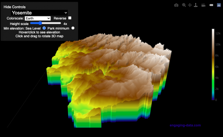
Play with an interactive 3D model of some popular National Parks in the US
I wanted to try my hand at creating 3D elevation models and thought trying to model some of the popular (and some of my favorite) national parks would be a good starting point.
Instructions
Once a 3D elevation model is selected and shown you can manipulated it in multiple ways:
- Zoom – You can zoom in and out, though the method depends on the device you are using. Try scrolling or pinch to zoom. You can also select the magnifying glass in the toolbar and drag to zoom.
- Rotate – You can rotate and change the angle of the model using by clicking and dragging on the model. This is the default selection in the toolbar (circular arrow around z axis)
- Pan – You can move the model around with if you select the panning tool from the toolbar (arrows going in all directions)
- Show contours – if you hover or click on part of the map, it can show all the areas of the model with the same elevation and the tooltip will show the geographic coordinates and elevation (you can toggle showing the tool tip if you select the tooltip bar)
- Save image – click on the camera icon in the toolbar to save as png
- Colors – you can change the color scale used to show elevation. You can also reverse the color scale.
- Change vertical exaggeration – you can select whether the vertical height is exaggerated using the ‘Height Scale’ slider. You can change between 1 (no exaggeration) to 11 (vertical scale is exaggerated by factor of 11).
- Change min elevation – you can select whether the minimum elevation is sea level or the lowest elevation in the park.
You can select a number of different parks from the drop down menu. If you have suggestions for additional parks, I may be able to add them to the list.
Note: the elevation files are data intensive since the visualization is downloading the elevation across in some cases, many hundreds or thousands of square miles. To keep the data needs down, I’ve reduced the resolution of the elevation data. Though the original data is 90 meter resolution (elevation is specified across every 90 x 90 m square in each park, I’ve averaged these squares together so that each park model only has about tens of thousands of these squares, regardless of the actual area of the park. This improves data loading and rendering times and makes the improves the responsiveness of the model.
Sources and Tools:
This visualization is written in HTML/CSS/Javascript. Digital elevation data is obtained from Open Topography and uses Shuttle Radar Topography Mission GL3 (90 meter resolution). The elevation data is downloaded using the opentopography API and parsed in a python script which downsamples the data to limit the number of elevation cells. The script also determines if a point is inside or outside of the park boundaries in order to create the elevation model. The 3D model is rendered using the Plotly open-source javascript graphing library.

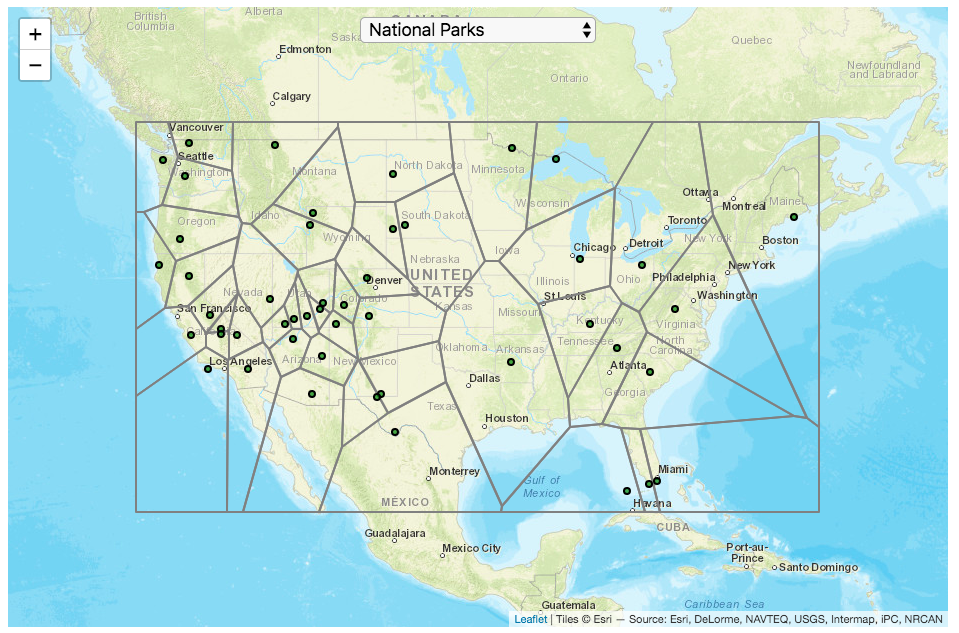
National Park Service Voronoi Map

This map divides up the Continental United States into different regions depending on which National Park (or other National Park Service site) is closest to it. It is based on a straight-line (‘as the crow flies’) distance between locations rather than along road networks. It is an example of a Voronoi Diagram, which is subdivided into different regions based upon the distance between points of interest. Everything within a subregion is closer to the point defining the region than any other point.
Hover over the circle points to see the name of the park. The map has a dropdown menu that lets you choose between the following types of locations in the National Park Service:
- National Parks
- National Historic Sites
- National Memorial Sites
- National Monuments
- National Seashores/Lakeshores
- National Recreation Areas
- National Battlefields
- National Military Sites
- National Scenic Areas
For National Parks, there is a high concentration of National Parks in the Western US, especially around the Southwestern US and running up the Pacific Coast. As a result, in these areas, the Voronoi regions are fairly small. The Southwest is also home to a high concentration of National Monuments. There are only few parks in the Eastern US and so the Voronoi regions are correspondingly large. Looking at National Historic Sites, the situation is flipped somewhat, with a high concentration of historic sites in the eastern US, and specifically the Northeast.
Let me know in the comments which park you are closest to and which park you last visited.
Tools and Data Sources
Locations of each of the National Park Service sites comes from the National Park Service. The map was created using the Leaflet javascript mapping library and the Voronoi diagram using the Turfjs javascript, geospatial analysis library.
National Park 3D Elevation Models
Play with an interactive 3D model of some popular National Parks in the US
I wanted to try my hand at creating 3D elevation models and thought trying to model some of the popular (and some of my favorite) national parks would be a good starting point.
Instructions
Once a 3D elevation model is selected and shown you can manipulated it in multiple ways:
- Zoom – You can zoom in and out, though the method depends on the device you are using. Try scrolling or pinch to zoom. You can also select the magnifying glass in the toolbar and drag to zoom.
- Rotate – You can rotate and change the angle of the model using by clicking and dragging on the model. This is the default selection in the toolbar (circular arrow around z axis)
- Pan – You can move the model around with if you select the panning tool from the toolbar (arrows going in all directions)
- Show contours – if you hover or click on part of the map, it can show all the areas of the model with the same elevation and the tooltip will show the geographic coordinates and elevation (you can toggle showing the tool tip if you select the tooltip bar)
- Save image – click on the camera icon in the toolbar to save as png
- Colors – you can change the color scale used to show elevation. You can also reverse the color scale.
- Change vertical exaggeration – you can select whether the vertical height is exaggerated using the ‘Height Scale’ slider. You can change between 1 (no exaggeration) to 11 (vertical scale is exaggerated by factor of 11).
- Change min elevation – you can select whether the minimum elevation is sea level or the lowest elevation in the park.
You can select a number of different parks from the drop down menu. If you have suggestions for additional parks, I may be able to add them to the list.
Note: the elevation files are data intensive since the visualization is downloading the elevation across in some cases, many hundreds or thousands of square miles. To keep the data needs down, I’ve reduced the resolution of the elevation data. Though the original data is 90 meter resolution (elevation is specified across every 90 x 90 m square in each park, I’ve averaged these squares together so that each park model only has about tens of thousands of these squares, regardless of the actual area of the park. This improves data loading and rendering times and makes the improves the responsiveness of the model.
Sources and Tools:
This visualization is written in HTML/CSS/Javascript. Digital elevation data is obtained from Open Topography and uses Shuttle Radar Topography Mission GL3 (90 meter resolution). The elevation data is downloaded using the opentopography API and parsed in a python script which downsamples the data to limit the number of elevation cells. The script also determines if a point is inside or outside of the park boundaries in order to create the elevation model. The 3D model is rendered using the Plotly open-source javascript graphing library.
National Park Service Voronoi Map
This map divides up the Continental United States into different regions depending on which National Park (or other National Park Service site) is closest to it. It is based on a straight-line (‘as the crow flies’) distance between locations rather than along road networks. It is an example of a Voronoi Diagram, which is subdivided into different regions based upon the distance between points of interest. Everything within a subregion is closer to the point defining the region than any other point.
Hover over the circle points to see the name of the park. The map has a dropdown menu that lets you choose between the following types of locations in the National Park Service:
- National Parks
- National Historic Sites
- National Memorial Sites
- National Monuments
- National Seashores/Lakeshores
- National Recreation Areas
- National Battlefields
- National Military Sites
- National Scenic Areas
For National Parks, there is a high concentration of National Parks in the Western US, especially around the Southwestern US and running up the Pacific Coast. As a result, in these areas, the Voronoi regions are fairly small. The Southwest is also home to a high concentration of National Monuments. There are only few parks in the Eastern US and so the Voronoi regions are correspondingly large. Looking at National Historic Sites, the situation is flipped somewhat, with a high concentration of historic sites in the eastern US, and specifically the Northeast.
Let me know in the comments which park you are closest to and which park you last visited.
Tools and Data Sources
Locations of each of the National Park Service sites comes from the National Park Service. The map was created using the Leaflet javascript mapping library and the Voronoi diagram using the Turfjs javascript, geospatial analysis library.
Recent Comments